Contents
- 1 Introduction
- 2 Requirements
- 2.1 Measuring
- 2.2 Analyzing
- 2.3 Generating test signals
- 3 Setting up the hardware
- 4 Setting up the software
- 4.1 Adding an XY graph
- 4.2 Add the I/O blocks
- 4.2.1 Differentiate I/O
- 4.2.2 Multiply I/O
- 4.2.3 Integrate I/O
- 4.3 Cursors
Introduction
In certain applications, the area that is enclosed by an XY graph needs to be determined. An example of this is determining the power loss in magnetic cores. When the flux density is plotted against the magnetic field intensity, the created XY graph will enclose a certain area, that is proportional to the power loss.
The area enclosed in an XY plot can be calculated as :
 |
or |  |
An oscilloscope measures both the X and Y signal as a function of time t. When incorporating that in the formulas, the area can be calculated using:
 |
or |  |
To implement this formula with an oscilloscope, one needs to differentiate one of the two signals, multiply it with the other signal and integrate the result of the multiplication. The amplitude difference in the result of the integration, during one period of one of the signals, is equal to the area enclosed in the XY graph.
Requirements
Measuring
To measure signals in XY mode, one needs an oscilloscope with at least two channels. For example the WiFiScope WS6 DIFF, WiFiScope WS6, WiFiScope WS5, WiFiScope WS4 DIFF, Handyscope HS6 DIFF, Handyscope HS5, Handyscope HS4 DIFF, Handyscope HS4 and the Handyscope HS3 are suitable instruments for measuring in XY mode.
Analyzing
The TiePie engineering Multi Channel oscilloscope software has several I/O blocks that can be used to process measured data. For this application, the Differentiate I/O, the Integrate I/O and the Multiply/Divide I/O will be used.
Generating test signals
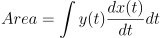
Any two signals can be measured and displayed in XY mode, but for demonstration purposes, this example uses two related signals, generated by a function generator with two output channels. The first signal is a square wave signal and the second signal is a triangular signal. Both signals have the same frequency and a constant phase difference. The signals are being measured with a Handyscope HS5.
Setting up the hardware
First the Handyscope HS5 is connected to the computer and the Multi Channel oscilloscope software is started.
Now connect Ch1 to one of the generator outputs and Ch2 to the other output of the generator.
Setting up the software
In our example, we are using a function generator to generate two signals. Both generate a -2 to +2 V signal. One is a square wave, the other is a triangular wave.
Input sensitivity, time base and trigger do not require special settings, just make sure that 2 to 3 cycles of the input signals are measured, in a suitable input range.
Adding an XY graph
When the Multi Channel oscilloscope software is started, it comes up with a Yt graph for the input channels of the connected instrument.
In this example we want to view both an Yt graph and an XY simultaneously, so an XY graph needs to be added.
Click the  XY mode button on the quick functions toolbar to create
a new graph with channel 1 versus channel 2.
XY mode button on the quick functions toolbar to create
a new graph with channel 1 versus channel 2.
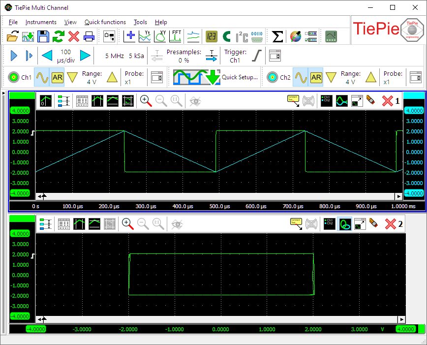
Add the I/O blocks
To perform the required calculations on the measured signals, a number of I/O blocks need to be created and connected. Refer to the article Creating and connecting objects for more information on this subject.
Differentiate I/O
The first operation in the calculation is to differentiate one of the two signals. In this example we will differentiate the signal on Ch2. Create a Differentiate I/O and connect the Ch2 to the Differentiate I/O.
Multiply I/O
The second operation in the calculation is to multiply the result of the differentiation with the other signal. Create a Multiply/Divide I/O connect the Differentiate I/O and Ch1 to the Multiply/Divide I/O. This I/O defaults to multiplying, so no settings need to be changed.
Integrate I/O
The last operation in the calculation is to integrate the result of the multiplication. Create an Integrate I/O and connect the Multiply/Divide I/O to it. Now drag the Integrate I/O to the graph with the Yt signals.
Cursors
The amplitude difference over one period of the input signals corresponds with the area enclosed by the XY graph.
Switch the vertical cursors on in the Yt graph with the
 Vertical cursors button and adjust one vertical cursor to mark the beginning of a period of the
signals and the other vertical cursor to mark the end of the same period of the input signals.
Vertical cursors button and adjust one vertical cursor to mark the beginning of a period of the
signals and the other vertical cursor to mark the end of the same period of the input signals.
In this example we're only interested in the 'Maximum-Minimum' measurement, so all other cursor measurements can be switched off. Note that the 'Right-Left' measurement will give the same result.
As you can see in the picture, the result of the measurement is indeed the enclosed area. You can verify this by counting the number of grid squares enclosed in the XY graph.