Contents
- 1 Object screen
- 1.1 Object tree
- 1.2 Object schema
The Multi Channel oscilloscope software has a modular structure, with measuring instruments, function generators and other objects constructed in the application. Besides measuring data with the TiePie engineering measuring instruments and displaying it like on a conventional scope, it is possible to do different kinds of processing on the measured data. Data can be combined with other measured data or with software generated data.
The objects that can be created, are divided into three groups:
-
 Sources: these objects generate data, like software generators.
Sources only have output(s) (like the channels of an instrument).
Sources: these objects generate data, like software generators.
Sources only have output(s) (like the channels of an instrument).
-
 I/Os: objects that accept data (Input), process this data in a specific way,
like e.g. adding, multiplying, filtering, etc. and then generate the processed data (Output).
These objects have input(s) and output(s).
I/Os: objects that accept data (Input), process this data in a specific way,
like e.g. adding, multiplying, filtering, etc. and then generate the processed data (Output).
These objects have input(s) and output(s).
-
 Sinks: these objects only accept data, like e.g. graphs and meters and tables.
These objects only have input(s).
Sinks: these objects only accept data, like e.g. graphs and meters and tables.
These objects only have input(s).
Objects can be combined and connected to each other to create measurement applications that range from very simple to very complex.
Object screen
Managing the objects and their connections is done in the Object screen.
The object screen is situated at the left side of the main window of the application.
It can be resized by dragging the splitter bar at the right of the object screen.
It can be revealed and hidden by clicking the
 Show object screen button on the main toolbar or by clicking the small triangle at the upper right corner of the
object screen.
In the application settings can be determined whether the object screen is default visible or hidden.
The status of the Object screen (visible or hidden) is also saved when a measurement is saved and restored when that
measurement is loaded again.
Show object screen button on the main toolbar or by clicking the small triangle at the upper right corner of the
object screen.
In the application settings can be determined whether the object screen is default visible or hidden.
The status of the Object screen (visible or hidden) is also saved when a measurement is saved and restored when that
measurement is loaded again.
The Object screen can be set to two different styles:
- as object tree
- as object schema
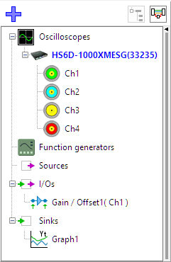
Object tree
The Object tree is a tree structure holding all objects, ordered by Instruments, Generators, Sources, I/Os and Sinks. It allows to add and remove objects and make connections between objects and setup objects.
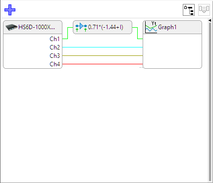
Object schema
The object schema is a schematic structure holding all objects. It shows all objects as blocks and shows all connections between the objects, making it easy to follow the data streams. It allows to add and remove objects and make connections between objects using easy drag and drop drawing techniques.