Digital data acquisition - Classroom

All digital oscilloscopes measure by sampling the analog input signals and digitizing the values.

Contents

1 Sampling
2 Sample frequency
2.1 Aliasing
3 Record Length
4 Timebase
5 Resolution

Sampling

When sampling the input signal, samples are taken at fixed intervals. At these intervals, the size of the input signal is converted to a number. The accuracy of this number depends on the resolution of the instrument. The higher the resolution, the smaller the voltage steps in which the input range of the instrument is divided. The acquired numbers can be used for various purposes, e.g. to create a graph.

Sampling

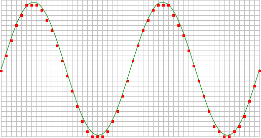
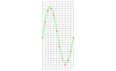
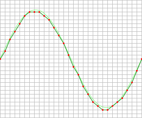
The sinewave in the above picture is sampled at the dot positions. By connecting the adjacent samples, the original signal can be reconstructed from the samples. You can see the result in the next illustration.

Connecting samples

Sample frequency

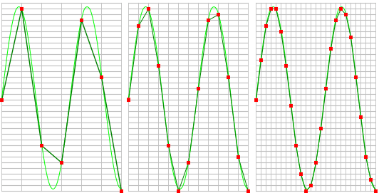
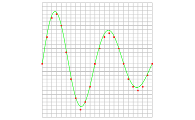
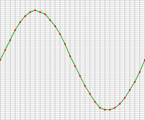
The rate at which the samples are taken is called the sampling frequency, the number of samples per second. A higher sampling frequency corresponds to a shorter interval between the samples. As is visible in the picture below, with a higher sampling frequency, the original signal can be reconstructed much better from the measured samples.

the effect of sampling frequency

The sampling frequency must be higher than 2 times the highest frequency in the input signal. This is called the Nyquist frequency. Theoretically it is possible to reconstruct the input signal with more than 2 samples per period. In practice, 10 to 20 samples per period are recommended to be able to examine the signal thoroughly.

Aliasing

When sampling an analog signal with a certain sampling frequency, signals appear in the output with frequencies equal to the sum and difference of the signal frequency and multiples of the sampling frequency. For example, when the sampling frequency is 1000 Hz and the signal frequency is 1250 Hz, the following signal frequencies will be present in the output data:

Multiple of sampling frequency	1250 Hz signal		-1250 Hz signal
...
-1000	-1000 + 1250 =	250	-1000 - 1250 =	-2250
0	0 + 1250 =	1250	0 - 1250 =	-1250
1000	1000 + 1250 =	2250	1000 - 1250 =	-250
2000	2000 + 1250 =	3250	2000 - 1250 =	750
...

As stated before, when sampling a signal, only frequencies lower than half the sampling frequency can be reconstructed. In this case the sampling frequency is 1000 Hz, so we can we only observe signals with a frequency ranging from 0 to 500 Hz. This means that from the resulting frequencies in the table, we can only see the 250 Hz signal in the sampled data. This signal is called an alias of the original signal.

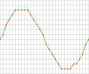
If the sampling frequency is lower than 2 times the frequency of the input signal, aliasing will occur. The following illustration shows what happens.

Aliasing

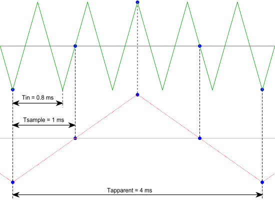
In this picture, the green input signal (top) is a triangular signal with a frequency of 1.25 kHz. The signal is sampled with a frequency of 1 kHz. The corresponding sampling interval is 1/( 1000 Hz ) = 1 ms. The positions at which the signal is sampled are depicted with the blue dots.

The red dotted signal (bottom) is the result of the reconstruction. The period time of this triangular signal appears to be 4 ms, which corresponds to an apparent frequency (alias) of 250 Hz (1.25 kHz - 1 kHz).

In practice, to avoid aliasing, always start measuring at the highest sampling frequency and lower the sampling frequency if required. Use function keys <F3> (lower) and <F4> (higher) to change the sampling fequency in a quick and easy way. The next illustration gives an example of what aliasing can look like.

Appearance of aliasing

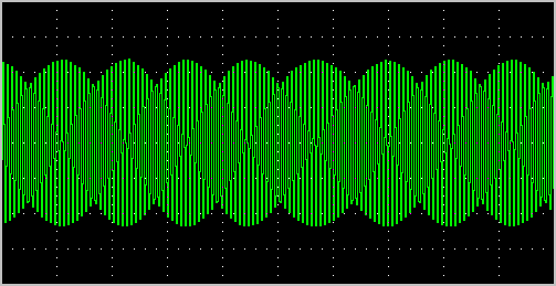
In this picture, a sine wave signal with a frequency of 257 kHz is sampled at a frequency of 50 kHz. The minimum sampling frequency for correct reconstruction is 514 kHz. For proper analysis, the sampling frequency should have been approximately 5 MHz.

Record Length

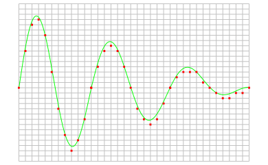
With a given sampling frequency, the number of samples that is taken determines the duration of the measurement. This number of samples is called record length. Increasing the record length, will increase the total measuring time. The result is that more of the measured signal is visible. In the images below, three measurements are displayed, one with a record length of 12 samples, one with 24 samples and one with 36 samples.

Record length 12 samples

Record length 24 samples

Record length 36 samples

The total duration of a measurement can easily be calculated, using the sampling frequency and the record length:

Measurement duration in seconds = record length in samples / sampling frequency in Hz

Use function keys <F11> (shorter) and <F12> (longer) to change the record length in a quick and easy way.

Timebase

The combination of sampling frequency and record length forms the time base of an oscilloscope. To setup the time base properly, the total measurement duration and the required time resolution have to be taken in account.

There are several ways to find the required time base setting. With the required measurement duration and sampling frequency, the required number of samples can be determined:

record length in samples = Measurement duration in seconds * sampling frequency in Hz

With a known record length in samples and the required measurement duration, the necessary sampling frequency can be calculated:

sampling frequency in Hz = record length in samples / Measurement duration in seconds

In the TiePie engineering software, both record length and sampling frequency can be set independently, to give the best flexibility. They can be selected from menu's, but also keyboard short cuts are available:

<F3> set the sampling frequency one step slower
<F4> set the sampling frequency one step faster
<F11> set the record length one step shorter
<F12> set the record length one step longer

Resolution

When digitizing the samples, the voltage at each sample time is converted to a number. This is done by comparing the voltage with a number of levels. The resulting number is the number of the highest level that's still lower than the voltage. The number of levels is determined by the resolution. The higher the resolution, the more levels are available and the more accurate the input signal can be reconstructed. In the image below, the same signal is digitized, using three different amounts of levels: 16, 32 and 64.

resolution 4 bits resolution 5 bits resolution 6 bits

The number of available levels, is determined by the resolution:

number of levels = 2 ^{resolution in bits}

The used resolutions in the previous image are respectively: 4 bits, 5 bits and 6 bits.

The Handyscope HS3, Handyscope HS4 and Handyscope HS4 DIFF can measure at four different resolutions: 8 bit (256 levels), 12 bit (4096 levels), 14 bit (16384 levels) and 16 bit (65536 levels).

The smallest detectable voltage difference depends on the resolution and the input range. This voltage can be calculated as:

minimum voltage = full scale range / number of levels

In the 200 mV range, the full scale ranges from -200 mV to +200 mV, the full range is 400 mV. When a 12 bit resolution is used, there are 2¹² = 4096 levels. This results in a smallest detectable voltage step of 0.400 V / 4096 = 97.7 µV. In 16 bit resolution this step is 0.400 V / 65536 = 6.1 µV